

Chasing a Blimp
Learning about weather radar through dirigibles

The following article is our monthly deep dive for paid subscribers. Our regular, free newsletters will resume next week.
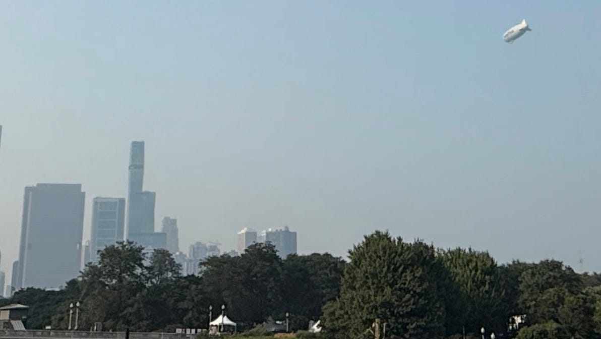
Recently, I spotted Ye Olde Goodyear Blimp flying over Chicago.
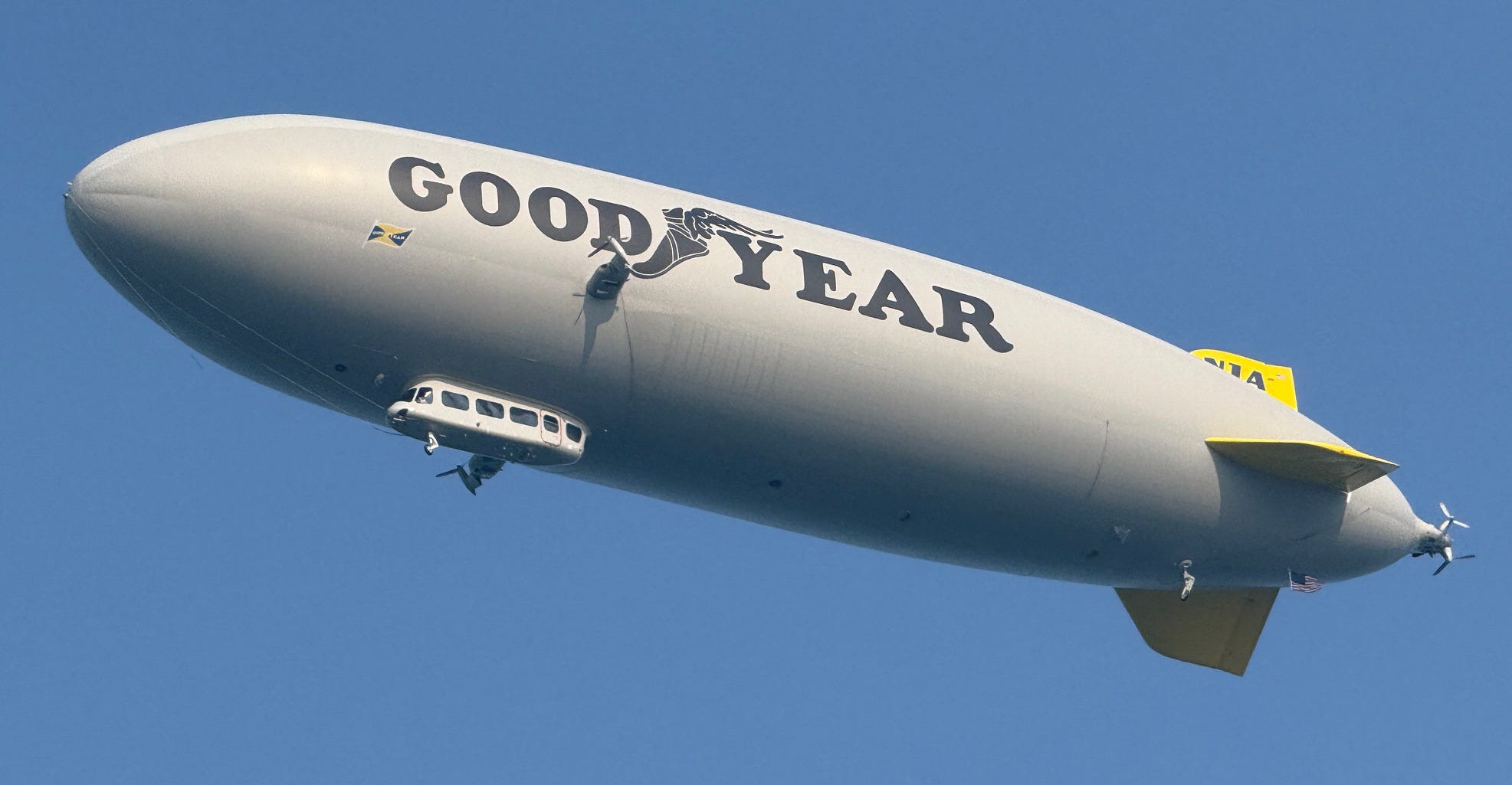
It was doing donuts over Lake Shore Drive, showing off to 100,000 drunk teenagers at Lollapalooza. Being more into weather than Weezer, I wondered whether we could detect the blimp on NWS radar. So I pulled up trusty Radarscope and also FlightRadar24.
The latter showed me the blimp’s path and altitude that afternoon.
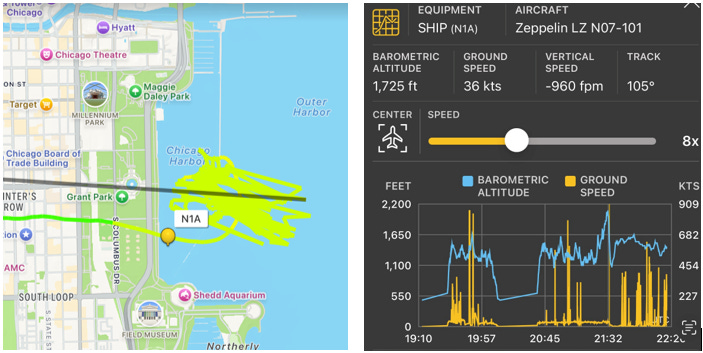
I asked ChatGPT whether it was plausible to detect the blimp that day, under those conditions, and at that altitude. It said it was possible but unlikely. The main issue was that the blimp would probably be flying below the radar beam.
The NWS Chicago weather radar station in Romeoville is 35 miles away. At its lowest elevation tilt angle of 0.5°, the bottom edge of the beam would be around 2,300 feet in altitude by the time it reached downtown Chicago1. As shown above, the blimp usually flies much lower than that. But its altitude spiked around 4:33 p.m. - coincidentally, when it arrived on station. My guess is that the crew took it higher to get some selfies before descending back to their cruising altitude.

The blimp’s peak altitude at 4:33 pm was about 2,200 feet. FlightRadar24’s data is compressed to fit the small chart. It’s possible the blimp could have been slightly higher than ~2,200 feet for brief intervals that don’t show up in the chart.
Radar beams aren’t hard-edged like lasers. They follow a pattern that closely resembles a Gaussian distribution of energy - strongest at the centerline and fading outward. Some fringe energy extends below the main beam. In rare cases, a large and reflective target (like a blimp) could be detected below the nominal edge of the beam’s pattern.
ChatGPT suggested which radar visualization (high-res reflectivity2) and elevation angle (0.5°) I should use. I fed them into RadarScope, let the gerbils run on the wheels, and…
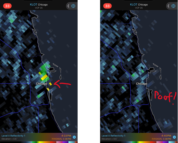
At 4:33 pm, a little yellow dot appears exactly where the blimp would have been at that moment in space and time. And it’s gone just a few minutes later. It’s true that the 4:33 p.m. image also shows other spots of enhanced reflectivity that later disappear. However, I can identify all of those as very tall buildings, ranging from 50 to 90 stories high, including that lone pixel to the south. That one belongs to a trio of lakeshore high-rises where one of my daughter’s best friends lives (her parents are very nice doctors). But trust me: there is no corresponding high rise in Lake Michigan.
Radar Scanning Modes

Note the label “VCP 35” at the top of the RadarScope frames. The NWS operates its radars using different scanning modes, each with strengths and weaknesses tailored to different weather situations. These are known as Volume Coverage Patterns (VCPs). The primary differences between the modes are the rate of rotation and the elevation angles employed. Slower rotation means more sensitivity, but takes longer. The angles they use have a strong influence over which parts of the sky they cover (see Jono Hey’s illustration above).
There are two categories of VCPs: Clear Air Mode and Precipitation Mode. NOAA describes them well:
As the name suggests, clear air mode is used when the weather is quiet. Instead of constantly scanning through all possible elevation angles, the radar antenna will slow down and scan fewer angles to reduce wear on the components. Once the radar detects precipitation while scanning in clear air mode, it will automatically switch over to precipitation mode. In precipitation mode, the radar antenna will speed up and scan 14 or 15 elevation angles, depending on the VCP in use.
In Clear Air Mode, there are two main scanning strategies: VCP 35 and VCP 31. In our case, RadarScope indicates that the radar was operating in VCP 35 mode - which is usually the default on calm, quiet days. It takes about 7 minutes for a radar to go through all its scans in VCP 35 mode. Sadly, we don’t know how long the blimp hovered around 2200ft. And it’s likely that it would only have been picked up by the 0.5° scan.
There was another time, about an hour later, when the blimp was raised above 2000ft again - though it didn’t get as high as 2200ft. I could find no signal in the radar during that event. But it could have simply missed the 0.5° scan, so its signal might have been drowned out in the background data of the longer scan.
Above is an animation showing about an hour of reflectivity over Chicago while in VCP 35 mode. Want to spot the tallest buildings in the city? That’s what the line up and down the lakefront represents. Also note two main clusters: one downtown and another farther south in Hyde Park/Jackson Park. As the animation progresses, only the tallest downtown buildings remain visible. That’s likely due to shifting atmospheric conditions in the early morning and their influence on how radar energy propagates3. The point here is to show just how variable radar sensitivity can be minute-to-minute.
Disappearing Data
RadarScope has the handy ability to pull up archival radar data. When I was writing this newsletter about a month later, I checked the archives to see if the blimp would show up in the velocity (Doppler) data. It wasn’t there. But, to my great surprise and confusion, the signal in the reflectivity data was now gone! I double-checked my settings to make sure I completely replicated the screenshots above. Something changed in the data between then and now. I noticed the time stamps are different, too. In the archival data, I can only pull up images from 4:28 pm and 4:35 pm. Whereas my screenshot was at 4:33 pm (which was a couple of hours after the radar scan was made). So the archival data is slightly different than the live data. Happily, I kept my receipts. Pro Tip: If you spot something unusual or interesting on a radar app or website, take a screenshot right away. It may not be there when you return to look later.
So did we detect the blimp? My gut puts the chances at 60%. The fact that we see a clear signal at the exact time and location of its greatest ascent (and no other time) is strong circumstantial evidence. On the other hand, it’s on the very edge of what is theoretically detectable. And it’s no longer in the archival data. It’s a close call! I wonder if I could get two meteorologists drunk and fighting over this? I’ll report back after the next AMS radar conference.
We are grateful to Lockheed Martin for a grant to support this newsletter. We acknowledge additional contributions from Dr. Milind Sharma.

Our archive of WWAT articles is here.
During the preparation of this work, the author(s) used ChatGPT-5 in order to copyedit text, calculate the beam width, and get recommendations for the radar search parameters. After using this tool, WWAT’s author(s) reviewed and edited the content as needed and take(s) full responsibility for the content of the publication.

Beam diameter ≈ 1.0° beam width × distance
Vertical beam width =
56,000⋅tan(0.5°)≈490 meters56,000 \cdot \tan(0.5°) ≈ 490 \, \text{meters}56,000⋅tan(0.5°)≈490meters
So the bottom edge of the beam is roughly:
950 m − 245 m ≈ 705 m AGL, or about 2,300 feet
Reflectivity is a visualization of backscattered power returned to the radar, not an actual mode of the radar.
A paraphrase from one of our scientific advisors: It's possible that there was ducting (aka super refraction) that led to the anomalous beam propagation towards the ground and intercepted the high-rise building[s]. That's one hypothesis to explain the enhanced clutter-like signature at 4:33 p.m. [and in the morning], but we cant know for sure. Ducting is strongly related to the refractive index of the atmospheric parcel being scanned and is most pronounced during the early morning hours due to erosion of low-level stability overnight as the solar insolation starts heating up the ground, leading to the formation of a daytime convective boundary layer.
Fascinating!